The World of Dimensionality Reduction

Dimensionality reduction is a major research/interest area for machine learning scientists/enthusiasts. It is basically a set of mathematical techniques which can use be used to make more sense of data. Imagine your boss at Amazon has given you a huge dataset of customer's buying habbits and activities on the website, and has asked you make sense of this huge pile of data being generated in process. Now there are multiple ways to go about it depending upon the exact outcome of the problem. For instance, lets say your're not really sure of how you'd like to approach the problem and you decide to apply some unsupervised learning techniques on your data, to organize it into clusters and groups in order to better understand the patterns. But, often times it could be hard if you're not really sure of what are you looking for, and you might need to make assumptions you aren't really comfortable with. We don't need to go into details about unsupervised learning algorithms today, lets save the best for the last. Before that its a good idea to first understand what really is dimensionality reduction and the intuition behind it.

As the name suggests, its a process to reduce the dimensions in the data. Lets go back to our Amazon example, where lets say the dataset given by your boss has 100 dimensions. This basically means each customer in the dataset, has 100 different fields or values assocaited with him like lets say location, age, gender etc. But when you consider all these dimensions or fields at the same time, it doesn't really tell you much, in the 100-dimension space. So its a good idea, to bring the dimensions down so that you can better understand your customers and try to identify the various degrees of freedom or the modes of variability. Its often a good idea to undertand the covariance of the data and try to identify the ways in which your data can high variance. This may all sound a little not too-familiar, so lets try to learn a few things before we dive deep into it. A good idea is to first understand what are vector spaces. If you're familiar with it, its okay to skip this post and move on to where we start discussing various dimensionality reduction techniques.

Before we proceed to discuss about Vector spaces, remember Dimensionality reduction is your friend and its an incredible tool to have in your arsenal to better understand and visualize your data, be it images or just news articles. Over the course of next few posts, we would discover various papers that were landmark in the field of dimensionality reduction and how exactly they acheive what they achieve. I'll try to make the post not math heavy, but I'll surely include all the proofs and mathematics that should help you understand the intuition. If you aren't familiar with vector spaces, I highly suggest to go through this brief post before we move on to the algorithms. Trust me, it'll make your life easier. So without further ado, lets checkout this beautiful world of vector spaces.

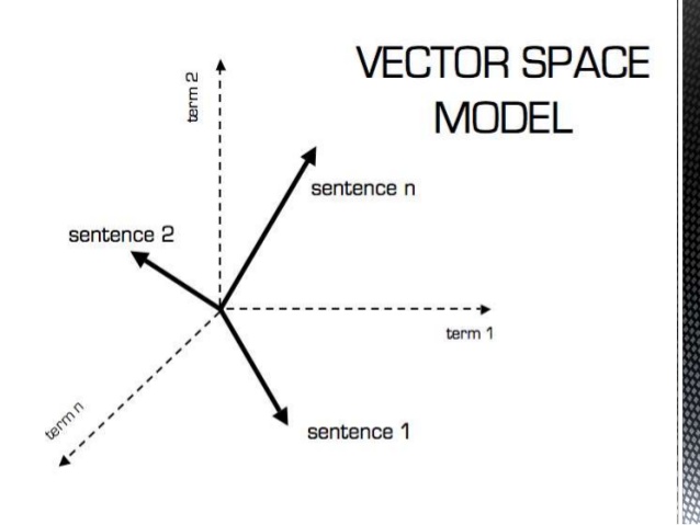
A vector space V is a collection (bag) of objects (vectors) that is closed under operations such as object (vector) addition and scalar (field F) multiplication, and it also needs to satisfy certain properties or axioms.

Axioms :
1) \( (\alpha + \beta)v = \alpha v + \beta v, \forall v \in \text{V and } \alpha, \beta \in F \)
2) \( \alpha(\beta v) = (\alpha\beta)v \)
3) \( u + v = v + u \text{ , where u,v } \epsilon V \)
4) \( u + (v + w) = (u + v) + w \text{ , where u,v,w } \epsilon V \)
5) \( \alpha(u + v) = \alpha u + \alpha v \)
6) \( \exists 0 \; \epsilon V \; \Rightarrow 0 + v = v \text{ ; 0 is usually called the origin or zero vector} \)
7) \( 0 v = 0 \)
8) \( e v = v \text{ , where e is the multiplicative unit in F} \)

Vectors in n-dimensions space, can be represented as n-dimensional tuple.
For example, \(R^n = {(a_1,a_2,...,a_n)|a_1,a_2,...a_n \; \epsilon \; R}\)

Let V be a vector space and U \( \subset \) V, we will call U a subspace of V, if U is also closed under vector addition, scalar multiplication and satisfies all other vector axioms.

For example, V = \(R^3 = {(a, b, c)|a, b, c \; \epsilon \; R}\)
U = \({(a, b, 0)|a, b \; \epsilon \; R}\)
Clearly U \( \subset \) V, and U is a subspace of V.

Let \( v_1,v_2 \epsilon R^3\) and W = \( {a v_1 + b v_2 | a, b \epsilon R} \) And W is a subspace of \( R^3\).
In this case, we say W is "spanned" by \( {v_1,v_2} \)
Okay, lets understand what is a span first.

In general, let S \( \subset \) V, where V is a vector space,and S has the form, S = \({v_1, v_2,...,v_k} \)

The span of the set S is the set U, where U \( \subset \) V. $$ U = { \sum_{j=1}^k a_j v_j | a_1,..., a_k \epsilon \;R } $$ Span is sometimes denoted like \( \mathcal{G}(v_1, v_2,...,v_k) \)

Linear Combination of Vectors
We say any vector (say u) is a linear combination of vectors (say \( v_1, v_2,..., v_3 \)), if it can be represented as \( u = a_1 v_1 + a_2 v_2 + ... + a_k v_k \text{ where} a_1,...,a_k are fields \).

Let S = {\( v_1, v_2,..., v_k \)} \(\subset\) V, a vector space. We say that S is linearly dependent if $$ a_1 v_1 + a_2 v_2 + ... + a_k v_k = 0 \text{ where not all coefficients are 0}$$ As you can see that any vector in this space can be represented as a linear combination of other vectors, therefore it has linear dependence (NOT LINEARLY INDEPENDENT).

The idea is to find a minimal generating set for a vector space.

Basically suppose V be a vector space, and S = {\( v_1, v_2, ..., v_k\)} is a linearly independent spanning set for V. Then S is called a basis of V.

Proof:
Clearly, V is spanned by S, as any vector in this vector space can be represented in the form of S. Important thing is to find out if S is linearly independent.
$$ 0 = a_1 e_1 + a_2 e_2 + a_3 e_3 $$ $$ (0, 0, 0) = a_1 (1, 0, 0) + a_2 (0, 1, 0) + a_3 (0, 0, 1) $$ $$ (0, 0, 0) = (a_1, a_2, a_3) $$ Hence, its linearly independent since, it is only 0, when all the coefficients together are 0, i.e., \( a_1=0, a_2=0, a_3=0 \)

The dimension of a vector space V is the number vectors in a basis of V.

Theorem:
Let S = {\( v_1, v_2,..., v_k\)} \( \subset \) V, be a basis for V, then every basis of V has k elements.
$$dim(R^n) = n $$ $$dim(P^n) = n + 1$$
Example: Let \( P^n = \) {\(a_n x^n + a_{n-1} x^{n-1} + ... + a_1 x^1 + a_0 x^0\)} be the vector space of polynomials of degree n. And so the powers <\( x^0, x^1, ..., x^n \)> they are linearly indpendent and they form a basis of \( P^n \). $$ P^n = \mathcal{G}(S) \text{ , where S = }(1, x, ..., x^n) $$

It is a way of putting a measure of distance on vector space.
Suppose that \( \left\|.\right\| \; V \rightarrow R^{+}\) is a function from V to the non-negative reals for which it needs to satisfy certain axioms.

Axioms: 1) \( \left\|v\right\| > 0 \; \forall v \in \text{V and } \left\|v\right\| = 0 \text{ if and only if } v = 0 \)
2) \( \left\| \alpha v\right\| = \alpha \left\| \ v\right\| \; \forall \alpha \in C, R and v \in V \)
3) \( \left\| u + v \right\| \leq \left\| u\right\| + \left\| v\right\| \forall v \in V\). This is the "triangular inequality"

Let V = \( R^n (or C^n) \). Define for x = (\( x_1, x_2, ..., x_n \) )
1) l2 norm : \( \left\|x\right\|_2 = (\left\lvert x_1 \right\rvert^2 + \left\lvert x_2 \right\rvert^2 + ... + \left\lvert x_n \right\rvert^2 )^{1/2} \)
2) l1 norm : \( \left\|x\right\|_1 = (\left\lvert x_1 \right\rvert + \left\lvert x_2 \right\rvert + ... + \left\lvert x_n \right\rvert ) \)
3) \( \left\|x\right\|_\infty = \max{1 \leq i \leq n} \; ( l_{\infty} norm )\)

Inner Product
Let F be the field, reals or complex numbers and V be a vector space over F. An inner product on V is a function, $$ (*, *) : v \; x \; v \; \rightarrow F $$ 1) (au + bv , cw) = a(u,w) + b(v,w) \( \forall a,b \in F and \forall \; u, v, w \in V \)
2) (u, v) = \( (\overline{u, v}) \; \forall u, v \in V \)
3) (v,v) > 0 , \( \forall \; \text{non-zero v} \in \) V
4) Also, define\( \left\|v\right\| = \sqrt{(v,v)} \)

Inner Product Space A vector space V over F with an inner product (*,*) is said to be an inner product space. Also knows as Hilber Space.
An inner product space V over Reals R is known as Euclidean Space whereas V over complex numbers C is known as unitary space.

Again, like vector spaces, it needs to satisy certain axioms.
Let F = R or C, and V be an inner product space over F. For v,w \( \in V \) and C \( \in \) F, we have :
1) \( \left\|c v\right\| = \left\lvert c \right\rvert \left\|v\right\| \)
2) \( \left\|c v\right\| > 0, \text{if v} \neq 0 \)
3) \( \left\lvert (u, v) \right\rvert \leq \left\|u\right\| \left\|v\right\| \)
This equality only holds true if and only if \( v = \frac{(u,v)}{\left\|v\right\|^2} v\). Also known as "Cauchy'Schwartz inequality"
4)\( \left\|u + v\right\| \leq \left\|u\right\| + \left\|v\right\|\).
Triangular Inequality holds true in Hilbert space as well.

Let V be an inner product space over the field F,
1) Suppose v,w \( \in \) V, then v & w are mutually orthogonal if the inner product |v,w| = 0
2) A subset S \( \in V\) is said to be an orthogonal set if v \( \perp \) w, \( \forall \) v, w \( \in \) S, and \( v \neq w \).
3) An orthogonal set S is said to be an orthogonal set if \( \left\|v\right\| = 1, \; \forall \; v \in \; S\)
4) Zero Vector is orthogonal to all elements of V.

Theorem 1:
Let V be an inner product space over F, and S be an orthogonal set of non-zero vectors. Then S is linearly indpependent.
Let V = \(R^n \) or V =\(C^n \). The the standard basis E = {\( e_1, e_2, ..., e_3\)} is an orthornormal set.