ISOMAP

A Global Geometric Framework for Non-linear Dimensionality Reduction - ISOMAP

Abstract:

Unlike classical dimensionality reduction techniques including principal component analysis (PCA) and multi-dimensional scaling (MDS), it tries to discover the non-linear degrees of freedom that underlies the complex natural observations, such as images of a face under different viewing conditions and handwriting data of a subject. ISOMAP computes a globally optimal solution, and for an important class of data manifolds, is guaranteed to converge asymptotically to true structure.

Definition of the problem:

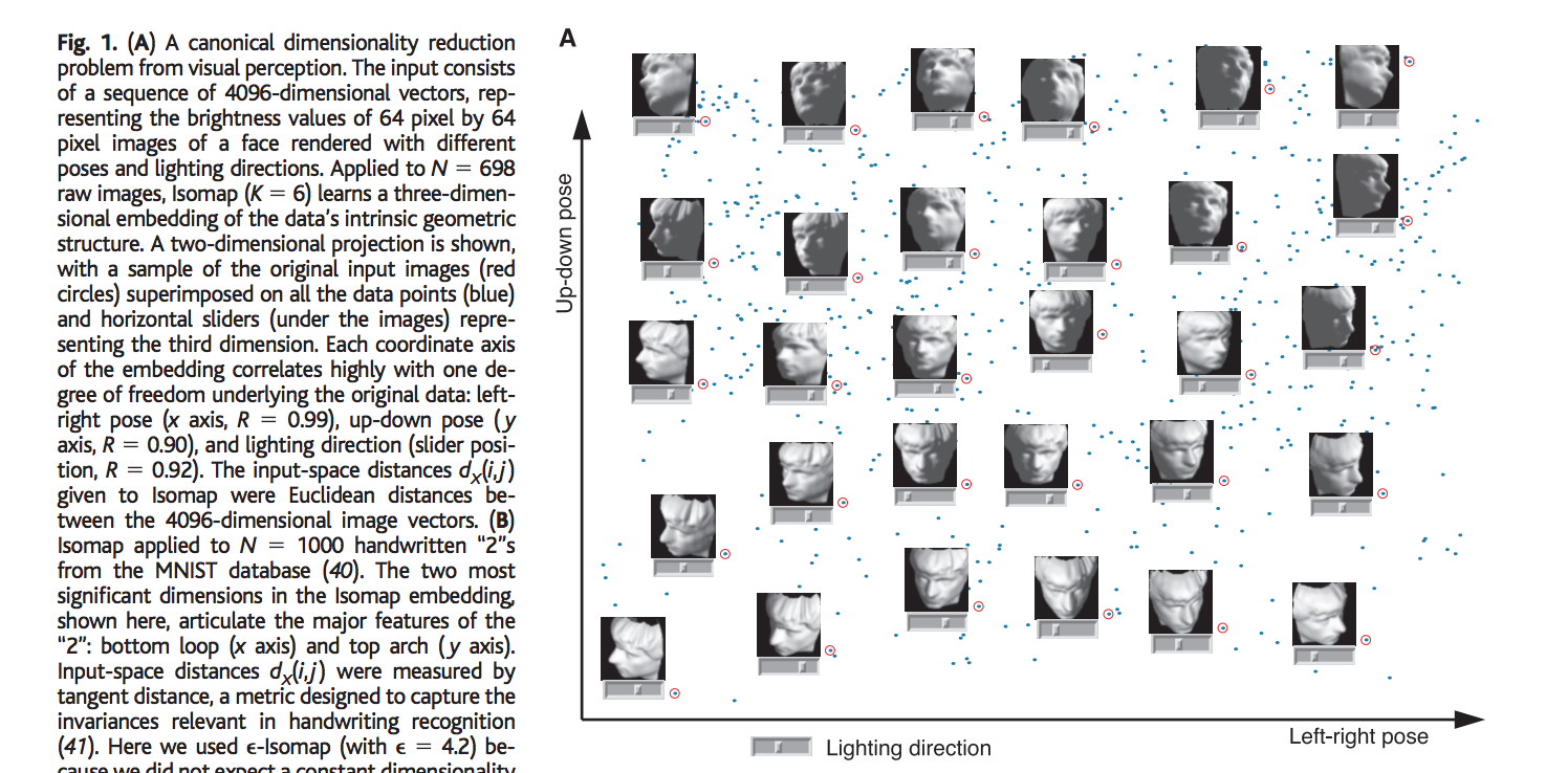
Let us consider the face dataset defined in the paper. The input consists of N images, where each image is a 64-by-64 pixels representation of pixels with 4096 dimensions. Each input dimension corresponding to the brightness level of one pixel in the image or the firing rate of one retinal ganglion cell. Even though the input is represented in this very high dimensional (4096-dim) space, the relevant meaningful structure of the image can be represented in much lower, 3 dimensional space. This lower dimensional meaningful structure corresponds to the independent degrees of freedom that lie on this intrinsic three dimensional manifold with the 4096 actual representation of the image. This 3-dim manifold can be parametrized by the two pose variables plus and azimuthal lightning angle. The primary goal of the algorithm in this problem is to discover this meaningful 3-dimensional lower representation (coordinates) that captures the intrinsic independent degrees of freedom of the dataset, from a given unordered higher 4096 dimensional original input space.

Comparison with other Dimensionality Reduction Techniques:

Other famous dimensionality reduction techniques include principal component analysis (PCA) and multi-dimensional scaling (MDSA) are simple to implement, efficiently computable and guaranteed to find the true structure of the data given that it lies on or near a linear subspace of the higher dimensional input space. PCA attempts to find a lower dimensional linear embedding which best preserves the variance of the input data in principal components (orthogonal axes to data). MDS finds an embedding which best preserves the pair wise distances between the points of higher dimensional input space, equivalent to PCA when the distances between points is Euclidean.

However, many of the real-world datasets contain essential non-linear structures that PCA and MDS can’t seem to identify and thus we need a technique which can discover these non-linear structures or the independent degrees of freedom. Comparing it to the face dataset example, PCA or MDS can’t identify the 3 intrinsic degrees of freedom (non-linear) of the dataset corresponding to the pose variables and the lighting, and thus would be a bad idea to represent this non-linear dataset in lower dimensional space.

However, ISOMAP technique combines the best algorithmic features of PCA and MDS–computational efficiency, global optimality and asymptotic convergence guarantees-with a flexibility to learn structures in a broad class of non-linear manifolds.

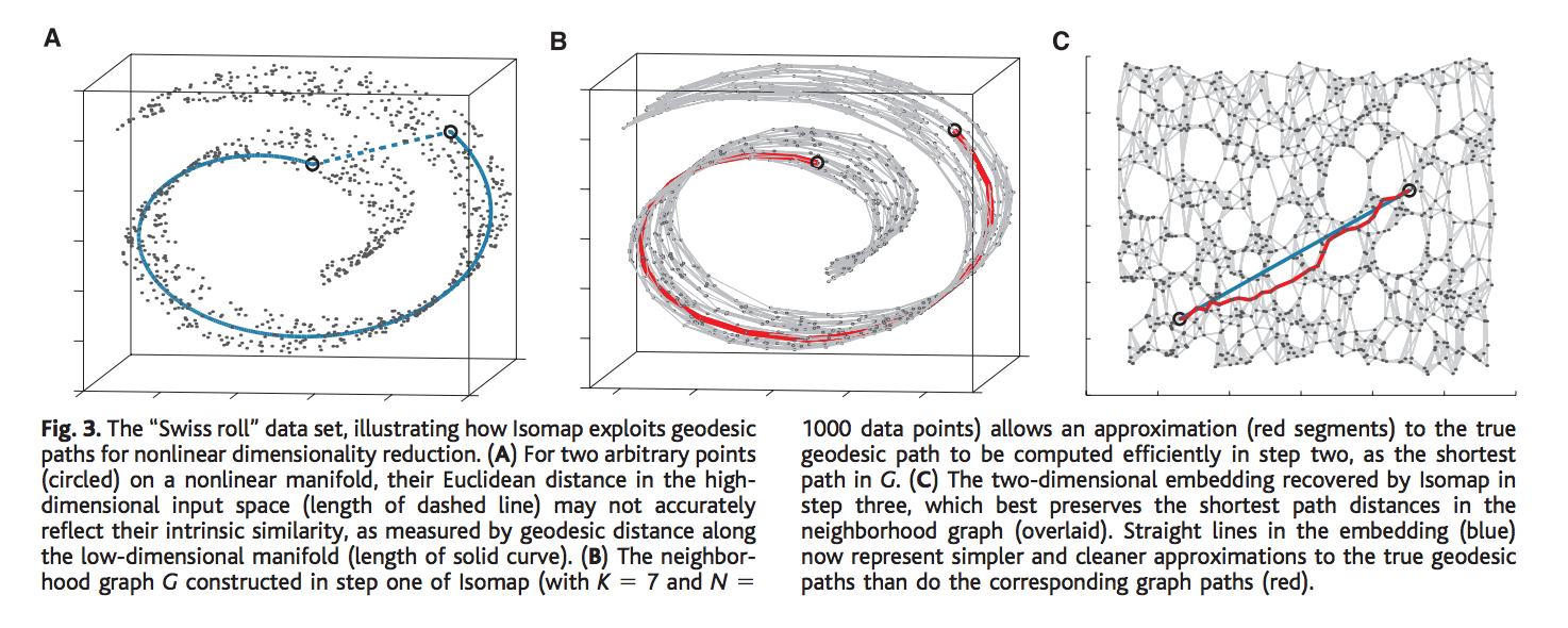
Let us see how PCA or MDS would fail to detect the intrinsic non-linear structure of property of a simple manifold with this “Swiss Roll manifold”. Given two points in the 3-dimensional manifold as represented by the two black circles, PCA or MDS would detect the shortest path distance between points based on Euclidean distance which seems like a very bad idea, as it would not be able to detect the underlying intrinsic geometric property or the distance between the points, i.e., it would not accurately reflect the relation between the points as it is in higher dimensional non-linear manifold. Imagine unrolling the swiss roll in a two-dimensional space, the two points which seems pretty close in 3-d space calculated using the Euclidean measure, are spread far apart in 2-d. Thus, Euclidean measure obviously fails to capture the intrinsic property of the manifold. We need a geodesic distance which in figure A, is denoted by the blue line. It accurately represents the actual distance between points on a non-linear manifold (manifold space).

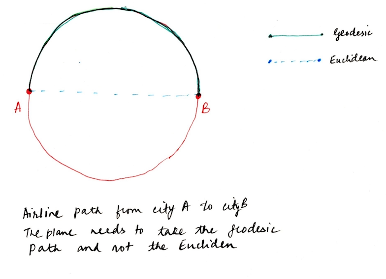
The intuition behind the Geodesic distance is easily captured if you consider the example of aerial/ground paths taken by airplanes/ships on earth. In order to go from city A to city B, it needs to take the Geodesic path which is denoted by the red path in the following figure. It is not possible for the plane/ship to take the smaller path(Euclidean) when we travel in the real-world. Similarly, on a non-linear manifold, the geodesic path represents the geometric structure much accurately compared to the Euclidean path.

The approach of ISOMAP builds on classical MDS,

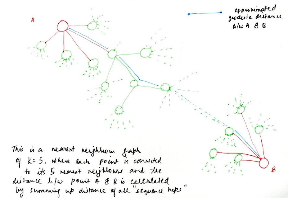
such that it works on the lines of capturing the essence of shortest path distances between all pair of points on the surface, but instead work with geodesic distances when working with manifolds. The most crucial point in this algorithm is estimating the geodesic distance between far-away points given only the input-space distances. For neighboring points, input-space distance provides a good approximate of geodesic points, and using this notion we can calculating the geodesic distances between faraway points by summing up the distances between the neighboring points. In other words, we capture the local metric information of the neighboring data points in order to come up to conclusions on points on a global level (points far away from each other), which give good approximations of the distances.

Algorithm

The complete isometric feature mapping or ISOMAP algorithm requires 3 steps.

Step 1: Construct a nearest neighbor graph for all the points in high dimensional input space.

This is the first step in the algorithm where we construct a nearest neighbor graph of all the data points in the higher dimensional input space based on their co-ordinates and the inter-distances. This can be done in two ways, choosing either the number of nearest neighbors K of each points or by choosing a value e, which basically denotes a value of some radius, and all the points that fall within e, are the nearest neighbors of some point.

In other words, define a Graph G over all the data points by connecting the points i and j if they are closer than e (e-Isomap), or if i is one of the K-nearest neighbors of j (K-Isomap). The closeness is measured by the distance between points i & j in the input space represented by d_x(i,j) and we can then set edge lengths of the nodes in G equal to d_x(i,j).

Step 2: Compute shortest paths

To compute the shortest path between the points on the graph G, we use a fairly simple algorithm called Floyd Warshall’s algorithm. It computes the shortest paths between all points in O(n³) time. The algorithm is as follows:

Algo:

1  let Dg be a |V| × |V| array of minimum distances initialized to ∞ (infinity)

2  for each vertex i

3     Dg[i][j] ← 0

4  for each edge (i,j)

5     Dg [i][j] ← dx(i,j)  // the weight of the edge (i,j)

6  for k from 1 to |V|

7     for i from 1 to |V|

8        for j from 1 to |V|

9           if Dg [i][j] > Dg [i][k] + Dg [k][j]

10              Dg [i][j] ← Dg [i][k] + Dg [k][j]

11          end if

Finally, the graph D_g will contain the shortest paths between all the points of the graph G.

Step 3: Construct d-dimensional embedding

This is the last and the most important step of the algorithm where we perform multi-dimensional scaling (MDS) to construct a lower d-dimensional embedding of the data.

Mutli-Dimensional Scaling(MDS)

• Technique that maps original high dimension space to lower dimensional space.
• MDS addresses the problem of constructing a configuration of t-points in an Euclidean space by using the information about the t-patterns. It preserves the pairwise distances.
• Although it has very different mathematics from PCA, it winds up being closely related and in fact yields a linear embedding.
• A t-by-t matrix is called a distance or affinity matrix if d_ii = 0 and d_ij > 0 where i ≠
• MDS tries to find the set of t points such that the distances between each pair of two points d_ij ^(X) (i & j points) in higher dimension X and the d_ij^(Y) in lower dimension Y are close to each other as possible. In other words, we need to find the a configuration of points in lower dimension such that the sum of difference between each pair of points is minimum.
• \( \min_{Y} \sum_{i = 1}^{t} \sum_{i = 1}^{t} (d_{ij}^{X} - d_{ij}^{Y})^2 \)
  

  where \( d_{ij}^{X} = \left\| X_i - X_j \right\|^2, X_i, X_j \)are points in input space X

  and \( d_{ij}^{X} = \left\| Y_i - Y_j \right\|^2 , Y_i, Y_j\)are points in lower dimensional space Y

• So basically MDS becomes an optimization problem where we need to find a configuration of t-point such the difference of the above summation gives us the minimum value.
• But the optimization equation above is the not the exact equation that we use. We need to perform a kernel trick and perform the optimization in the inner product space, often known as Hilbert space if it’s a complete inner product space. The intuition is to project our points in inner product higher dimensional space where it is much easier to separate the data points (becomes linearly separable).
• So the distance matrix is then converted to a kernel matrix of inner products X^TX by $$ X^T X = \frac{-1}{2} H D^{(X)} H $$ $$ where \; H = 1 - \frac{1}{t} e e^T \text{ and e is a column vector of all 1s}$$

• Now the final equation that we need to optimize is $$ \min_{Y} \sum_{i = 1}^{t} \sum_{i = 1}^{t} (X_i^{T} X_i - Y_i^{T} Y_i)^2 $$
• Finally, the solution is $$ Y = \Lambda^{\frac{1}{2}} V^T $$ $$ \text{where V is the top d eigen vectors of} X^T X$$ $$ \text{where } \; \Lambda \text{is the top d eigen values of} X^T X$$
• The global minimum is achieved by setting the coordinates (y_i) in Y space, to the top d Eigen vectors of the matrix (X^TX) where X is the distance matrix D^G.
• Solution of MDS is very identical to dual PCA. Also, as far as Euclidean distance is concerned, PCA and MDS produce the same results. However, distances need not based on Euclidean distances, and thus can represent many types of dissimilarities between objects (example, the approximated geodesic distance in the face dataset was able to differentiate between various independent degrees of freedom).

Conclusions

• ISOMAP guarantees a global optimum and is also guaranteed asymptotically to recover the true dimensionality and geometric structure of a strictly larger class of non-linear manifolds. Like the swiss roll example above, there are many non-linear manifolds whose intrinsic geometry is that of a convex region in Euclidean space, but whose ambient geometry in high dimensional data is very folded, twisted or curved. For non-Euclidean manifolds, such as a hemisphere or the surface of the donut, ISOMAP is still able to produce a globally optimum low-dimensional Euclidean representation.
• These guarantees of asymptotic convergence rests on a proof that as the number of data point increases, the graph distances D_g(i,j) provide increasingly better approximations to the intrinsic geodesic distances D_M(i,j),  becoming arbitrarily accurate in the limit of the input data. How quickly D_g(i,j)  converges to D_M(i,j),  depends on a number on certain parameters of the manifold as it lies within high dimensional space (radius of curvature and branch separation) and on the density of points.
• Isomap’s global coordinates provide a simple way to analyze and manipulate high dimensional observations in terms of their intrinsic non-linear degrees of freedom.

For example, in the face dataset, Isomap was able to separate the true underlying factors that the made the dataset and separated them in a way, that it was easy to understand non-linear structure of the data.

• The problem with Isomap is that computationally very expensive if we a large dataset, considering how expensive it can be compute shortest paths between all pair of data points.

Implementation & Comparison of different Dimensionality Reduction Techniques

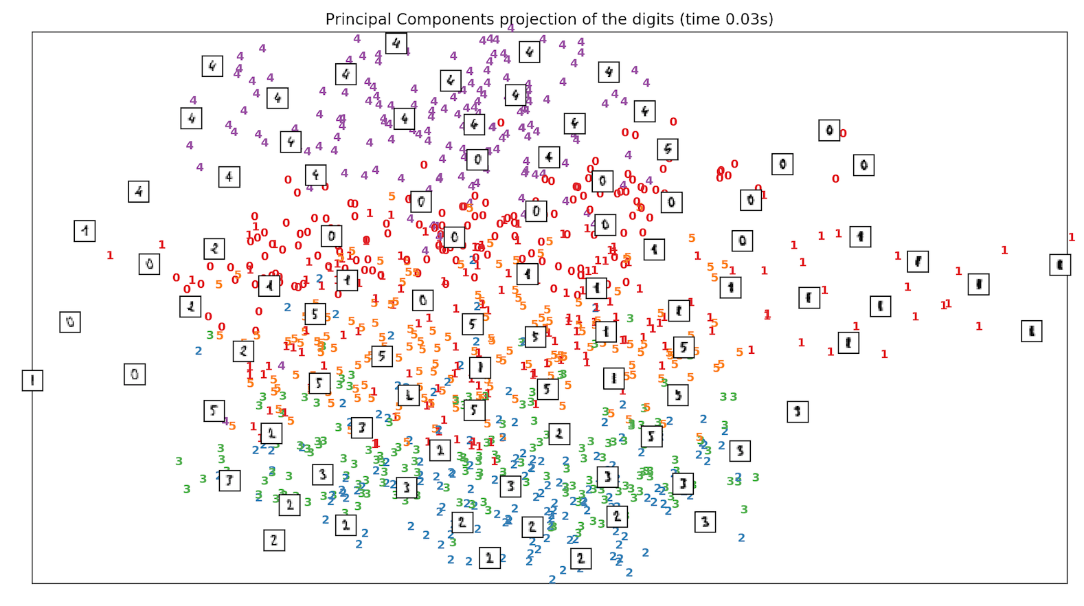
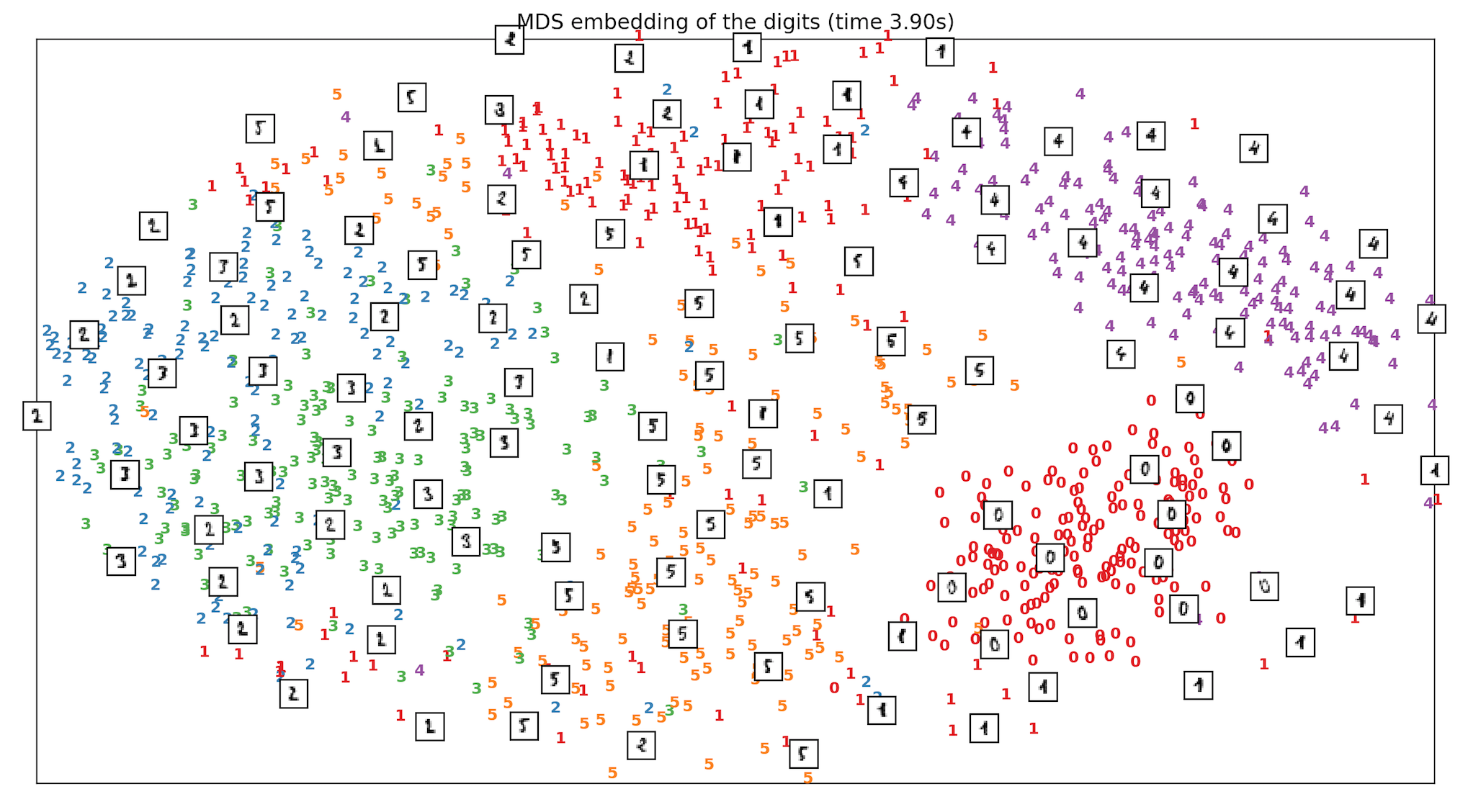
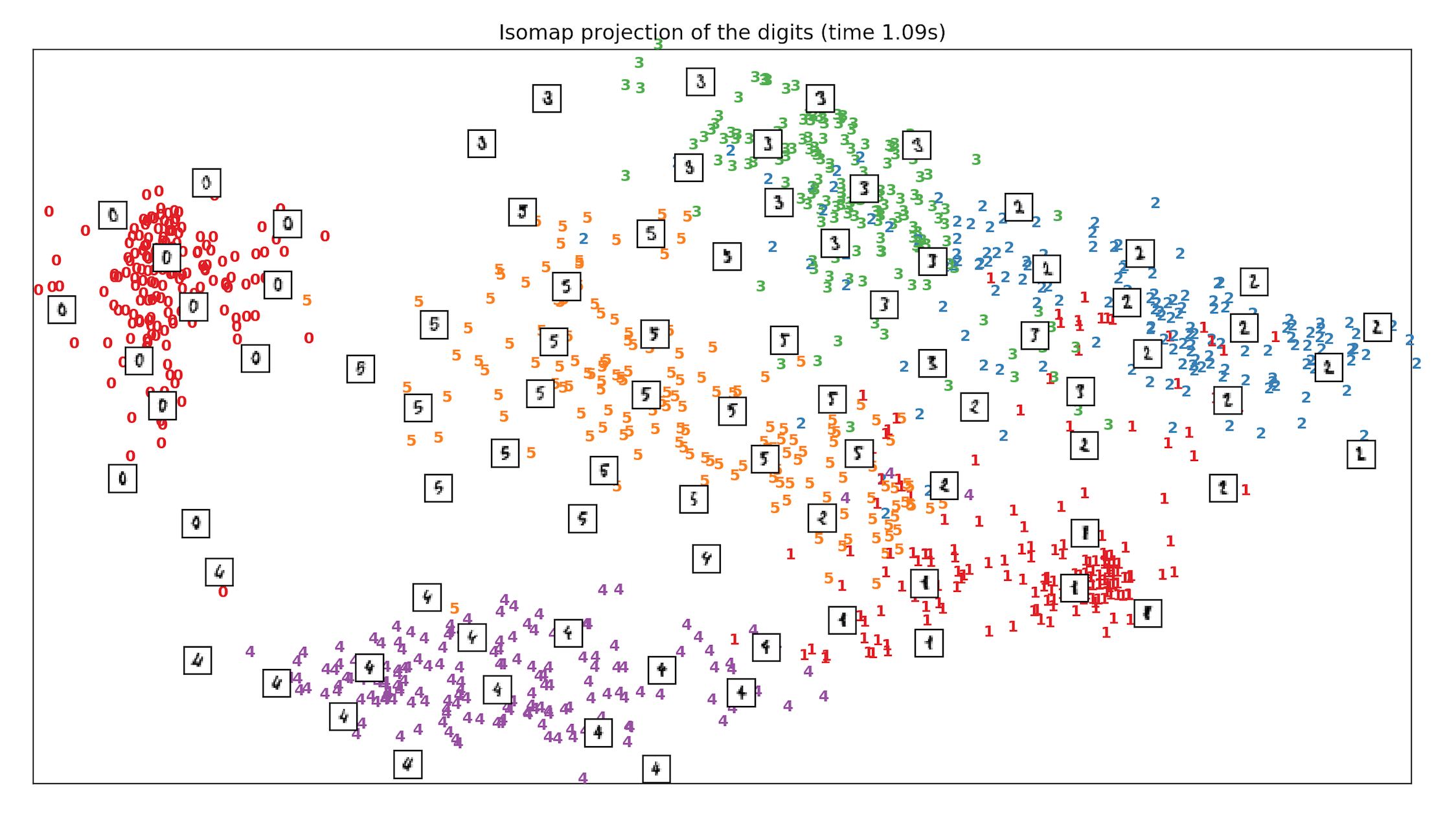
• We run and test the Handwritten digits dataset of classes from digit 0 to digit 5 and see how different techniques including PCA, MDS & ISOMAP compare when it comes to separation of classes, in Sklearn. ISOMAP is the clear winner.

SKLEARN CODE:

from time import time
from sklearn import (manifold, datasets, decomposition, ensemble, discriminant_analysis, random_projection)
import numpy as np 
import matplotlib.pyplot as plt 
from matplotlib import offsetbox

#load the dataset 
digits = datasets.load_digits(n_class=6)
X = digits.data
y = digits.target
n_samples, n_features = X.shape
n_neighbors = 30
#scale and visualize the embedding vectors
def plot_embedding(X, title=None):
    x_min, x_max = np.min(X, 0), np.max(X, 0)
    X = (X - x_min) / (x_max - x_min)

    plt.figure()
    ax = plt.subplot(111)
    for i in range(X.shape[0]):
        plt.text(X[i, 0], X[i, 1], str(digits.target[i]),
                 color=plt.cm.Set1(y[i] / 10.),
                 fontdict={'weight': 'bold', 'size': 9})

    if hasattr(offsetbox, 'AnnotationBbox'):
        # only print thumbnails with matplotlib > 1.0
        shown_images = np.array([[1., 1.]])  # just something big
        for i in range(digits.data.shape[0]):
            dist = np.sum((X[i] - shown_images) ** 2, 1)
            if np.min(dist) < 4e-3:
                # don't show points that are too close
                continue
            shown_images = np.r_[shown_images, [X[i]]]
            imagebox = offsetbox.AnnotationBbox(
                offsetbox.OffsetImage(digits.images[i], cmap=plt.cm.gray_r),
                X[i])
            ax.add_artist(imagebox)
    plt.xticks([]), plt.yticks([])
    if title is not None:
        plt.title(title) 
# Plot images of the digits 
#arrange them in an order to form one image which shows all the digits
n_img_per_row = 20
img = np.zeros((10 * n_img_per_row, 10 * n_img_per_row))
for i in range(n_img_per_row):
    ix = 10 * i + 1
    for j in range(n_img_per_row):
        iy = 10 * j + 1
        img[ix:ix + 8, iy:iy + 8] = X[i * n_img_per_row + j].reshape((8, 8))

plt.imshow(img, cmap=plt.cm.binary)
plt.xticks([])
plt.yticks([])
plt.title('A selection from the 64-dimensional digits dataset')

def main():
	# Projection on to the first 2 principal components
	print("Computing PCA projection")
	t0 = time()
	X_pca = decomposition.TruncatedSVD(n_components=2).fit_transform(X)
	plot_embedding(X_pca,
	               "Principal Components projection of the digits (time %.2fs)" %
	               (time() - t0))

	# MDS  embedding of the digits dataset
	print("Computing MDS embedding")
	clf = manifold.MDS(n_components=2, n_init=1, max_iter=100)
	t0 = time()
	X_mds = clf.fit_transform(X)
	print("Done. Stress: %f" % clf.stress_)
	plot_embedding(X_mds,
	               "MDS embedding of the digits (time %.2fs)" %
	               (time() - t0))

	# Isomap projection of the digits dataset
	print("Computing Isomap embedding")
	t0 = time()
	X_iso = manifold.Isomap(n_neighbors, n_components=2).fit_transform(X)
	print X_iso.shape
	print("Done.")
	plot_embedding(X_iso,
	               "Isomap projection of the digits (time %.2fs)" %
	               (time() - t0))
	plt.show()
main()

Outcome