Local Linear Embeddding

Motivation:

The need to analyze multivariate data in almost every major field in science, raises the fundamental problem of dimensionality reduction: how to discover compact representations of high-dimensional data. Local Linear Embedding is one such unsupervised algorithm which addresses this problem, by computing low-dimensional embedding’s that preserves the local geometry of the of the data, i.e., the neighborhood embedding’s of the high dimensional data. It basically belongs to the class of algorithms which take the approach of Think Globally, Fit Locally. Local Linear Embedding maps its inputs into a single global co-ordinate system of lower dimensionality, and its optimizations don’t involve local minima. It basically tries to learn the global structure of non-linear manifolds, such as those generated by images of faces, or documents of text, by exploiting the local symmetries of linear constructions.

How different from other Dimensionality Reduction techniques?

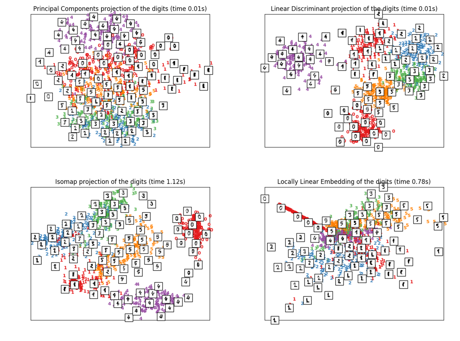
PCA and MDS try to identify the various degrees of freedom by considering the variances and the pairwise distances amongst all points in the dataset, respectively. But both fail to identify the underlying structure of the manifold properly because they map far away data points on the manifold to nearby points in the plane, which gives us the wrong information about the geometry of the manifold. More sophisticated methods such as ISOMAP does a much better job when it comes to mapping points that are far way on the manifold to a plane, but it also requires us to compute pairwise distances between all the points on the non-linear manifold. This can cause big problems when the structure of the manifold is complicated and we have to sample a large number of points in order to correctly reconstruct it. ISOMAP gives increasingly worse performance with more data points, as we would still be required to compute the pairwise distances between them. And if we sample less points, in order to increase our efficiency, it can lead us to construct a bad picture of the manifold that we need to work with. That’s why LLE, is such a good algorithm to work with as we don’t really need to compute any sort of pairwise distances. It tries to preserve the non-linear global structure by working with local linear patches on the manifold and then later combine all its findings to build a global presentation or structure.

Algorithm:

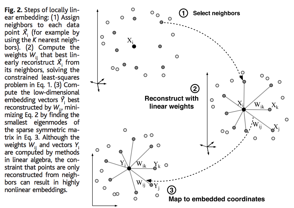
Step 1: Construct a k-nearest neighbor graph of points locally. Select neighbors of point \( X_i \).

Step 2: Reconstruct the point \( X_i \) as a linear combination of weights \( W_ij \) for all j nearest neighbors of \( X_i \) $$ \overline{X_i} = W_{i1} X_1 + W_{i2} X_2 + ... + W_{ij} X_j $$ We do this by optimizing an objective function, $$ \epsilon(W) = \min_{i = 1}^{t} \left\| X_i - \sum_{j = 1}^{k} W_{ij} X_j \right\|^2$$ Step 3: Map to the lower dimensional space by using these linear weights W, that were learned from the previous step and identfy/learn these lower-d Y cordinates, using another objective function, $$ \phi(Y) = \sum_{j = 1}^{t} \left\| Y_i - \sum_{j = 1}^{t} W_{ij} Y_j \right\|^2 $$

Summary:

• The algorithm only requires us to go through a single pass of the steps in the algorithm and finds us the global minima of the reconstruction and the embedding costs.

• Many popular learning algorithms don’t share the favorable properties of LLE. Iterative hill climbing methods for auto-encoder neural networks , self-organizing maps and latent variable models don’t have the same guarantees of global optimality or convergence. They also tend to involve many more free parameters, such as learning rates, convergence criteria and architectural specifications.

• Other non-linear DR methods rely on deterministic annealing schemes to avoid local minima, the optimizations of LLE are especially tractable.

• It is computationally much faster than methods like ISOMAP, where we need to perform dynamic programming in order to compute the shortest path of the geodesic distances.

• Also, LLE scales very well with the intrinsic manifold dimensionality d, and doesn’t require a discretized gridding of the embedding space. This basically means that as more dimensions are added to the embedding space, the existing ones don’t change, so the LLE doesn’t have to be re-rerun to compute higher dimensional embeddings.

• The best aspect about LLE is the possibility of its usage in a diverse set of problems in different areas of science because of its less number of assumptions and free parameters. It works well with images and documents of words where it can even identify semantic association of words and thus building a global coordinate system where similar words are close to each other.

In the next post of Local Linear Embedding, we will prove all the equations and see how we solve the optimization problem in LLE.

References: